Project Part I

The trends in alcohol consumption

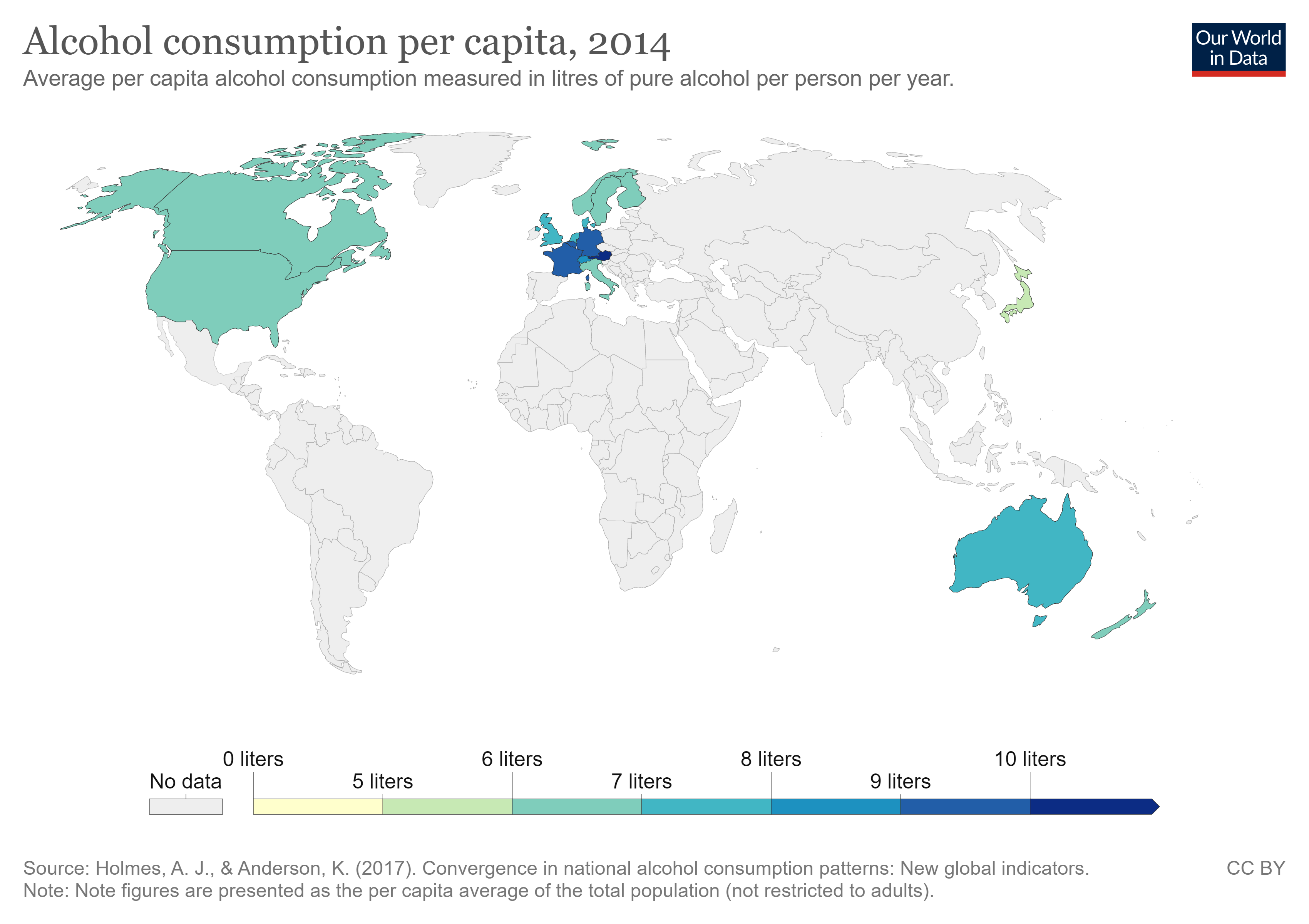
1. I downloaded the Alcohol consumption data from Our World in Data. I selected this data because I’m interested in observing alcohol consumption for high income countries.

---

2. This is the link to the data.

3. These are the R packages I will use to read and prepare data for analysis.

library(tidyverse)
library(here)

4. Read data into R.

file_csv <- here("_posts", "2022-05-02-project-part-i", "per-capita-alcohol-1890.csv")

alcohol.1 <- read_csv(file_csv)

---

5. Use glimpse to glimpse the data to see names and columns.

glimpse(alcohol.1)

Rows: 121
Columns: 4
$ Entity                                                      <chr> ~
$ Code                                                        <chr> ~
$ Year                                                        <dbl> ~
$ `Alcohol consumption since 1890 (Alexander & Holmes, 2017)` <dbl> ~

---

6. Prepare data for analysis.

• Change the name of the first column from Entity to Country

• Change name of fourth column from Alcohol consumption since 1890 (Alexander & Holmes, 2017) to Ounces

• Use mutate to convert from litres to Ounces

• Assign output to consumption

• Display consumption

consumption <- alcohol.1 %>%
rename(Country = Entity, Ounces = `Alcohol consumption since 1890 (Alexander & Holmes, 2017)`) %>% 
  select(Country, Year, Ounces) %>% 
  mutate(Ounces = Ounces * 33.81)

consumption

# A tibble: 121 x 3
   Country    Year Ounces
   <chr>     <dbl>  <dbl>
 1 Australia  1890   199.
 2 Australia  1920   128.
 3 Australia  1960   240.
 4 Australia  1970   321.
 5 Australia  1980   328.
 6 Australia  1990   274.
 7 Australia  2000   274.
 8 Australia  2014   247.
 9 Austria    1960   294.
10 Austria    1970   365.
# ... with 111 more rows

---

• Find the mean alcohol consumption for 1990.

• Start with consumption THEN

• filter for the year 1990 THEN

• Find the mean alcohol consumption for that year.

consumption %>% 
  filter(Year == 1990) %>% 
  summarize(mean(Ounces))

# A tibble: 1 x 1
  `mean(Ounces)`
           <dbl>
1           277.

• The mean alcohol consumption for high income countries in 1990 was 277 Oz. per capita.

---

• Find the mean alcohol consumption for 2000.

• Start with consumption THEN

• filter for year 2000 THEN

• Find the mean alcohol consumption for that year.

consumption %>% 
  filter(Year == 2000) %>% 
  summarize(mean(Ounces))

# A tibble: 1 x 1
  `mean(Ounces)`
           <dbl>
1           269.

• The mean alcohol consumption for high income countries in 2000 was 269 Oz. per capita.

• Alcohol consumption per capita decreased from 1990 to 2000 for high income countries.

---

7. Add a picture

Distribution by country

---

8. Write the data to file in the project directory.

write_csv(consumption, file = "consumption.csv")