Load the R packages that we will use

library(tidyverse)
library(infer)
library(skimr)

Question: t-test

Set random seed generator to 123
Load data into R, assign it to hr

set.seed(123)

hr <- read_csv("https://estanny.com/static/week13/data/hr_2_tidy.csv",
               col_types = "fddfff")

Use skim to summarize the data in hr

skim(hr)

Table 1: Data summary
Name	hr
Number of rows	500
Number of columns	6
_______________________
Column type frequency:
factor	4
numeric	2
________________________
Group variables	None

Variable type: factor

skim_variable	complete_rate	ordered	n_unique	top_counts
gender	1	FALSE	2	mal: 256, fem: 244
evaluation	1	FALSE	4	bad: 154, fai: 142, goo: 108, ver: 96
salary	1	FALSE	6	lev: 95, lev: 94, lev: 87, lev: 85
status	1	FALSE	3	fir: 194, pro: 179, ok: 127

Variable type: numeric

skim_variable	n_missing	complete_rate	mean	sd	p0	p25	p50	p75	p100	hist
age	0	1	39.86	11.55	20.3	29.60	40.2	50.1	59.9	▇▇▇▇▇
hours	0	1	49.39	13.15	35.0	37.48	45.6	58.9	79.9	▇▃▂▂▂

The mean hours worked per week is 49.4.

Is the mean number of hours worked per week 48?

specify that hours is the variable of interest.

hr %>% 
  specify(response = hours)

Response: hours (numeric)
# A tibble: 500 x 1
   hours
   <dbl>
 1  78.1
 2  35.1
 3  36.9
 4  38.5
 5  36.1
 6  78.1
 7  76  
 8  35.6
 9  35.6
10  56.8
# ... with 490 more rows

hypothesize that the average hours worked is 48

hr %>% 
  specify(response = hours) %>% 
  hypothesize(null = "point", mu = 48)

Response: hours (numeric)
Null Hypothesis: point
# A tibble: 500 x 1
   hours
   <dbl>
 1  78.1
 2  35.1
 3  36.9
 4  38.5
 5  36.1
 6  78.1
 7  76  
 8  35.6
 9  35.6
10  56.8
# ... with 490 more rows

generate 1000 replicates representing the null hypothesis

hr %>% 
  specify(response = hours) %>% 
  hypothesize(null = "point", mu = 48) %>% 
  generate(reps = 1000, type = "bootstrap")

Response: hours (numeric)
Null Hypothesis: point
# A tibble: 500,000 x 2
# Groups:   replicate [1,000]
   replicate hours
       <int> <dbl>
 1         1  39.7
 2         1  44.3
 3         1  46.8
 4         1  33.7
 5         1  39.6
 6         1  39.5
 7         1  40.5
 8         1  55.8
 9         1  72.6
10         1  35.7
# ... with 499,990 more rows

The output has 500,000 rows

calculate the distribution of statistics from the generated data
- assign output to null_t_distribution
- display null_t_distribution

null_t_distribution <- hr %>%
  specify(response = age) %>% 
  hypothesize(null = "point", mu = 48) %>% 
  generate(reps = 1000, type = "bootstrap") %>% 
  calculate(stat = "t")

null_t_distribution

Response: age (numeric)
Null Hypothesis: point
# A tibble: 1,000 x 2
   replicate     stat
       <int>    <dbl>
 1         1  0.144  
 2         2 -1.72   
 3         3  0.404  
 4         4 -1.11   
 5         5  0.00894
 6         6  1.46   
 7         7 -0.905  
 8         8 -0.663  
 9         9  0.291  
10        10  3.09   
# ... with 990 more rows

null_t_distribution has 1000 t-stats.

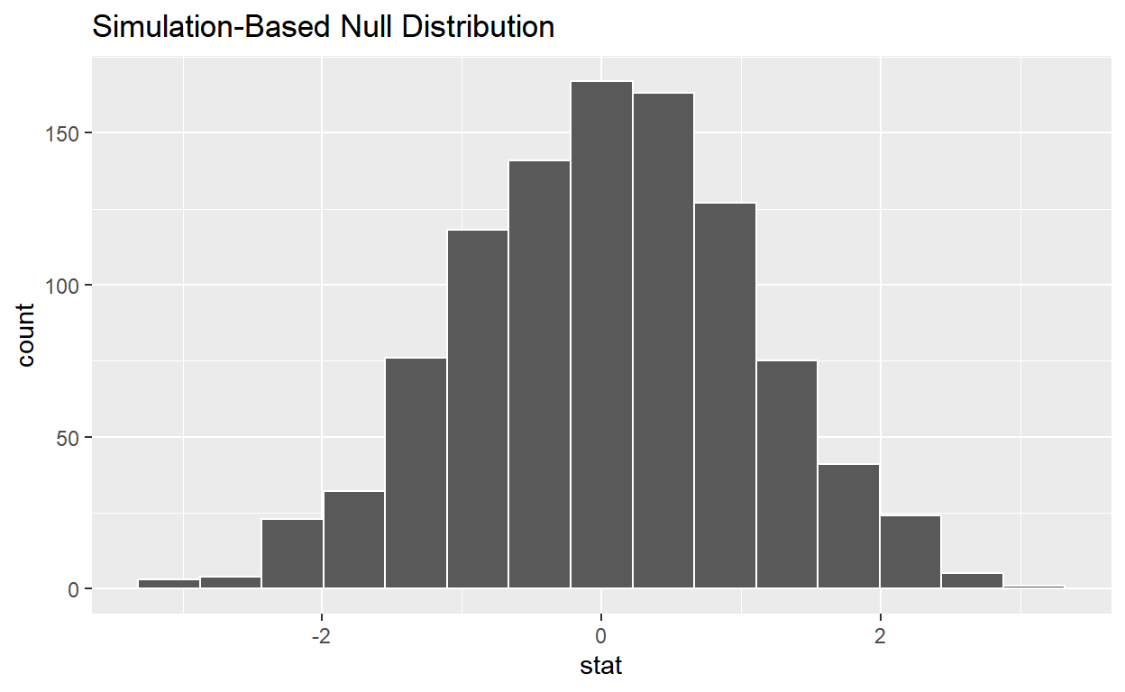
visualize the simulated null distribution.

visualise(null_t_distribution)

calculate the statistic from your observed data.
- assign the output to observed_t_statistic
- display observed_t_statistic

observed_t_statistic <- hr %>% 
  specify(response = hours) %>% 
  hypothesize(null = "point", mu = 48) %>% 
  calculate(stat = "t")

observed_t_statistic

Response: hours (numeric)
Null Hypothesis: point
# A tibble: 1 x 1
   stat
  <dbl>
1  2.37

get_p_value from the simulated null distribution and the observed statistic.

null_t_distribution %>% 
  get_p_value(obs_stat = observed_t_statistic, direction = "two-sided")

# A tibble: 1 x 1
  p_value
    <dbl>
1   0.014

shade_p_value on the simulated null distribution.

null_t_distribution %>% 
  visualize() +
  shade_p_value(obs_stat = observed_t_statistic, direction = "two-sided")

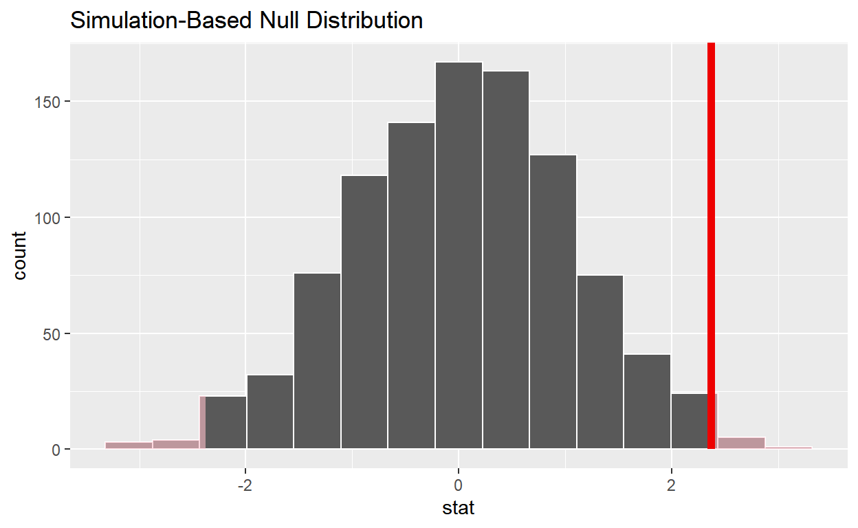
Is the p-value < 0.05? yes
Does your analysis support the null hypothesis that the true mean number of hours worked was 48? no

Question: Sample t-test 2

Load data into R, assign it to hr_2

hr_2 <- read_csv("https://estanny.com/static/week13/data/hr_1_tidy.csv",
                 col_types = "fddfff")

Is the average number of hours worked the same for both genders in hr_2?

Use skim to summarize the data in hr_2 by gender.

hr_2 %>% 
  group_by(gender) %>% 
  skim()

Table 2: Data summary
Name	Piped data
Number of rows	500
Number of columns	6
_______________________
Column type frequency:
factor	3
numeric	2
________________________
Group variables	gender

Variable type: factor

skim_variable	gender	complete_rate	ordered	n_unique	top_counts
evaluation	female	1	FALSE	4	fai: 81, bad: 71, ver: 57, goo: 51
evaluation	male	1	FALSE	4	bad: 82, fai: 61, goo: 55, ver: 42
salary	female	1	FALSE	6	lev: 54, lev: 50, lev: 44, lev: 41
salary	male	1	FALSE	6	lev: 52, lev: 47, lev: 46, lev: 39
status	female	1	FALSE	3	fir: 96, pro: 87, ok: 77
status	male	1	FALSE	3	fir: 89, ok: 76, pro: 75

Variable type: numeric

skim_variable	gender	complete_rate	mean	sd	p0	p25	p50	p75	p100	hist
age	female	1	41.78	11.50	20.5	32.15	42.35	51.62	59.9	▆▅▇▆▇
age	male	1	39.32	11.55	20.2	28.70	38.55	49.52	59.7	▇▇▆▇▆
hours	female	1	50.32	13.23	35.0	38.38	47.80	60.40	79.7	▇▃▃▂▂
hours	male	1	48.24	12.95	35.0	37.00	42.40	57.00	78.1	▇▂▂▁▂

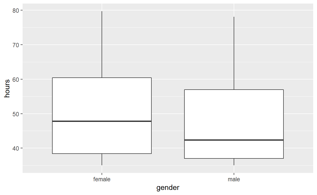
Females worked an average of 50.3 hours per week.
Males worked an average of 48.2 hours per week.

Use geom_boxplot to plot distribution of hours worked by gender.

hr_2 %>% 
  ggplot(aes(x = gender, y = hours)) +
  geom_boxplot()

specify the variables of interest are hours and gender

hr_2 %>% 
  specify(response = hours, explanatory = gender)

Response: hours (numeric)
Explanatory: gender (factor)
# A tibble: 500 x 2
   hours gender
   <dbl> <fct> 
 1  36.5 female
 2  55.8 female
 3  35   male  
 4  52   female
 5  35.1 male  
 6  36.3 female
 7  40.1 female
 8  42.7 female
 9  66.6 male  
10  35.5 male  
# ... with 490 more rows

hypothesize that the number of hours worked and gender are independent.

hr_2 %>%
  specify(response = hours, explanatory = gender) %>% 
  hypothesize(null = "independence")

Response: hours (numeric)
Explanatory: gender (factor)
Null Hypothesis: independence
# A tibble: 500 x 2
   hours gender
   <dbl> <fct> 
 1  36.5 female
 2  55.8 female
 3  35   male  
 4  52   female
 5  35.1 male  
 6  36.3 female
 7  40.1 female
 8  42.7 female
 9  66.6 male  
10  35.5 male  
# ... with 490 more rows

generate 1000 replicates representing the null hypothesis

hr_2 %>%
  specify(response = hours, explanatory = gender) %>% 
  hypothesize(null = "independence") %>% 
  generate(reps = 1000, type = "permute")

Response: hours (numeric)
Explanatory: gender (factor)
Null Hypothesis: independence
# A tibble: 500,000 x 3
# Groups:   replicate [1,000]
   hours gender replicate
   <dbl> <fct>      <int>
 1  36.4 female         1
 2  35.8 female         1
 3  35.6 male           1
 4  39.6 female         1
 5  35.8 male           1
 6  55.8 female         1
 7  63.8 female         1
 8  40.3 female         1
 9  56.5 male           1
10  50.1 male           1
# ... with 499,990 more rows

The output has 500,000 rows.

calculate the distribution of statistics from the generated data.
- Assign output to null_distribution_2_sample_permute
- Display null_distribution_2_sample_permute

null_distribution_2_sample_permute <- hr_2 %>%
  specify(response = hours, explanatory = gender) %>% 
  hypothesize(null = "independence") %>% 
  generate(reps = 1000, type = "permute") %>% 
  calculate(stat = "t", order = c("female", "male"))

null_distribution_2_sample_permute

Response: hours (numeric)
Explanatory: gender (factor)
Null Hypothesis: independence
# A tibble: 1,000 x 2
   replicate   stat
       <int>  <dbl>
 1         1 -0.208
 2         2 -0.328
 3         3 -2.28 
 4         4  0.528
 5         5  1.60 
 6         6  0.795
 7         7  1.24 
 8         8 -3.31 
 9         9  0.517
10        10  0.949
# ... with 990 more rows

null_t_distribution has 1000 t-stats.

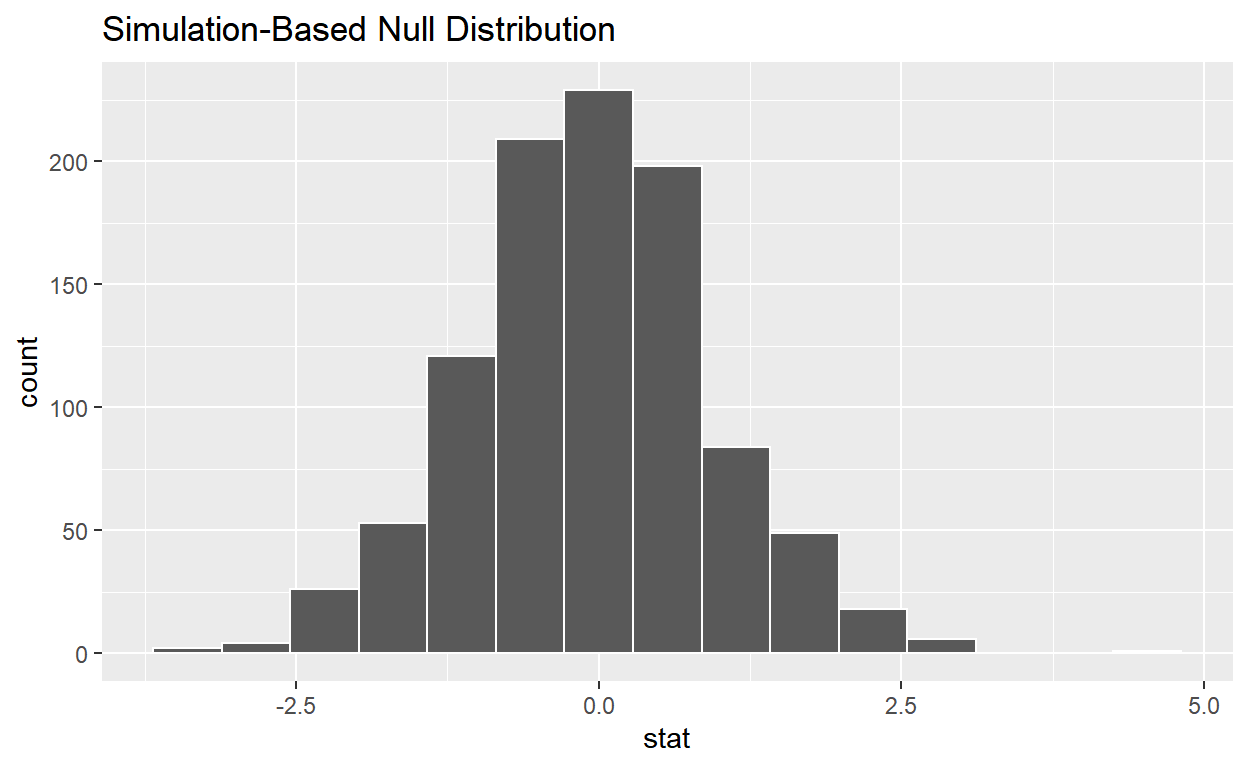
visualize the simulated null distribution.

visualize(null_distribution_2_sample_permute)

calculate the statistic from your observed data.
- Assign the output to observed_t_2_sample_stat
- Display observed_t_2_sample_stat

observed_t_2_sample_stat <- hr_2 %>% 
  specify(response = hours, explanatory = gender) %>% 
  calculate(stat = "t", order = c("female", "male"))

observed_t_2_sample_stat

Response: hours (numeric)
Explanatory: gender (factor)
# A tibble: 1 x 1
   stat
  <dbl>
1  1.78

get_p_value from your simulated null distribution and the observed statistic

null_t_distribution %>% 
  get_p_value(obs_stat = observed_t_2_sample_stat, direction = "two-sided")

# A tibble: 1 x 1
  p_value
    <dbl>
1   0.086

shade_p_value on the simulated null distribution.

null_t_distribution %>% 
  visualize() +
  shade_p_value(obs_stat = observed_t_2_sample_stat, direction = "two-sided")

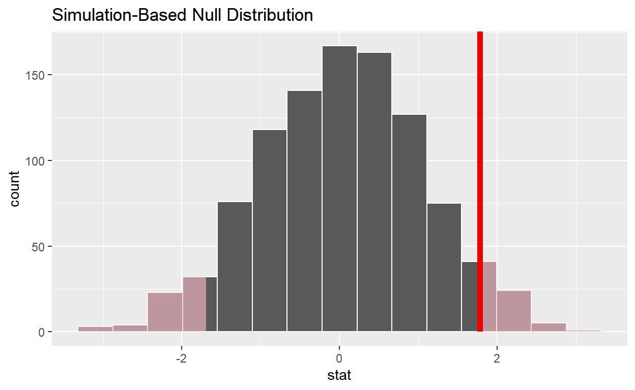
Is the p-value < 0.05? no
Does your analysis support the null hypothesis that the true mean number of hours worked by female and male employees was the same? yes

Question: ANOVA

Load data into R, assign to hr_anova

hr_anova <- read_csv("https://estanny.com/static/week13/data/hr_2_tidy.csv",
                     col_types = "fddfff")

Is the average number of hours worked the same for all three status (fired, ok, & promoted)?

Use skim to summarize the data into hr_anova by status

hr_anova %>% 
  group_by(status) %>% 
  skim()

Table 3: Data summary
Name	Piped data
Number of rows	500
Number of columns	6
_______________________
Column type frequency:
factor	3
numeric	2
________________________
Group variables	status

Variable type: factor

skim_variable	status	complete_rate	ordered	n_unique	top_counts
gender	promoted	1	FALSE	2	mal: 90, fem: 89
gender	fired	1	FALSE	2	fem: 101, mal: 93
gender	ok	1	FALSE	2	mal: 73, fem: 54
evaluation	promoted	1	FALSE	4	goo: 70, ver: 62, fai: 24, bad: 23
evaluation	fired	1	FALSE	4	bad: 78, fai: 72, goo: 25, ver: 19
evaluation	ok	1	FALSE	4	bad: 53, fai: 46, ver: 15, goo: 13
salary	promoted	1	FALSE	6	lev: 42, lev: 42, lev: 39, lev: 34
salary	fired	1	FALSE	6	lev: 54, lev: 44, lev: 34, lev: 24
salary	ok	1	FALSE	6	lev: 32, lev: 31, lev: 26, lev: 19

Variable type: numeric

skim_variable	status	complete_rate	mean	sd	p0	p25	p50	p75	p100	hist
age	promoted	1	40.63	11.25	20.4	30.75	41.10	50.25	59.9	▆▇▇▇▇
age	fired	1	40.03	11.53	20.3	29.45	40.40	50.08	59.9	▇▅▇▆▆
age	ok	1	38.50	11.98	20.3	28.15	38.70	49.45	59.9	▇▆▅▅▆
hours	promoted	1	59.21	12.66	35.0	49.75	58.90	70.65	79.9	▅▆▇▇▇
hours	fired	1	41.67	8.37	35.0	36.10	38.45	43.40	77.7	▇▂▁▁▁
hours	ok	1	47.35	10.86	35.0	37.10	45.70	54.50	78.9	▇▅▃▂▁

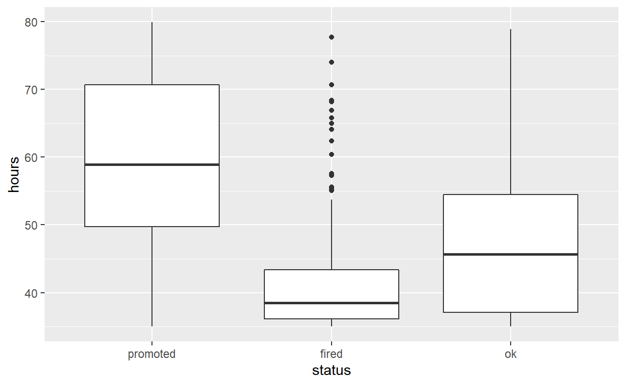
Employees that were fired worked an average of 41.7 hours per week.
Employees that were ok worked an average of 47.4 hours per week.
Employees that were promoted worked an average of 59.2 hours per week.

Use geom_boxplot to plot distributions of hours worked by status.

hr_anova %>% 
  ggplot(aes(x = status, y = hours)) +
  geom_boxplot()

specify the variables of interest are hours and status

hr_anova %>% 
  specify(response = hours, explanatory = status)

Response: hours (numeric)
Explanatory: status (factor)
# A tibble: 500 x 2
   hours status  
   <dbl> <fct>   
 1  78.1 promoted
 2  35.1 fired   
 3  36.9 fired   
 4  38.5 fired   
 5  36.1 fired   
 6  78.1 promoted
 7  76   promoted
 8  35.6 fired   
 9  35.6 ok      
10  56.8 promoted
# ... with 490 more rows

hypothesize that the number of hours worked and status are independent.

hr_anova %>%
  specify(response = hours, explanatory = status) %>% 
  hypothesise(null = "independence")

Response: hours (numeric)
Explanatory: status (factor)
Null Hypothesis: independence
# A tibble: 500 x 2
   hours status  
   <dbl> <fct>   
 1  78.1 promoted
 2  35.1 fired   
 3  36.9 fired   
 4  38.5 fired   
 5  36.1 fired   
 6  78.1 promoted
 7  76   promoted
 8  35.6 fired   
 9  35.6 ok      
10  56.8 promoted
# ... with 490 more rows

generate 1000 replicates representing the null hypothesis

hr_anova %>%
  specify(response = hours, explanatory = status) %>% 
  hypothesise(null = "independence") %>% 
  generate(reps = 1000, type = "permute")

Response: hours (numeric)
Explanatory: status (factor)
Null Hypothesis: independence
# A tibble: 500,000 x 3
# Groups:   replicate [1,000]
   hours status   replicate
   <dbl> <fct>        <int>
 1  41.9 promoted         1
 2  36.7 fired            1
 3  35   fired            1
 4  58.9 fired            1
 5  36.1 fired            1
 6  39.4 promoted         1
 7  54.3 promoted         1
 8  59.2 fired            1
 9  40.2 ok               1
10  35.3 promoted         1
# ... with 499,990 more rows

The output has 500,000 rows.

calculate the distribution of statistics from generated data
- Assign the output to null_distribution_anova
- Display null_distribution_anova

null_distribution_anova <- hr_anova %>%
  specify(response = hours, explanatory = status) %>% 
  hypothesise(null = "independence") %>% 
  generate(reps = 1000, type = "permute") %>% 
  calculate(stat = "F")

null_distribution_anova

Response: hours (numeric)
Explanatory: status (factor)
Null Hypothesis: independence
# A tibble: 1,000 x 2
   replicate  stat
       <int> <dbl>
 1         1 0.312
 2         2 2.85 
 3         3 0.369
 4         4 0.142
 5         5 0.511
 6         6 2.73 
 7         7 1.06 
 8         8 0.171
 9         9 0.310
10        10 1.11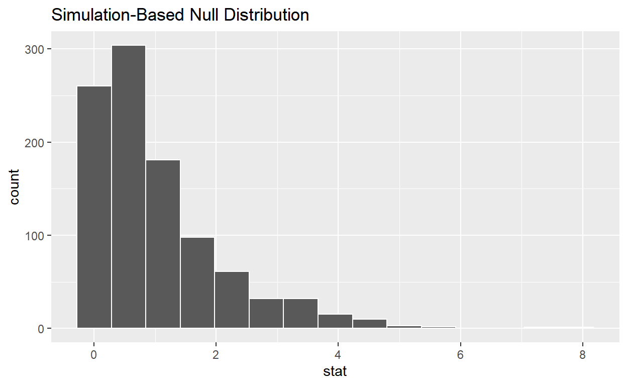 
# ... with 990 more rows

null_distribution_anova has 1000 F-stats.

visualize the statistic from your observed data.

visualise(null_distribution_anova)

calculate the statistic from your observed data.
- Assign the output to observed_f_sample_stat
- Display observed_f_sample_stat

observed_f_sample_stat <- hr_anova %>% 
  specify(response = hours, explanatory = status) %>% 
  calculate(stat = "F")

observed_f_sample_stat

Response: hours (numeric)
Explanatory: status (factor)
# A tibble: 1 x 1
   stat
  <dbl>
1  128.

get_p_value from the simulated null distribution and the observed statistic.

null_distribution_anova %>% 
  get_p_value(obs_stat = observed_f_sample_stat, direction = "greater")

# A tibble: 1 x 1
  p_value
    <dbl>
1       0

shade_p_value on the simulated null distribution.

null_t_distribution %>% 
  visualize() +
  shade_p_value(obs_stat = observed_f_sample_stat, direction = "greater")

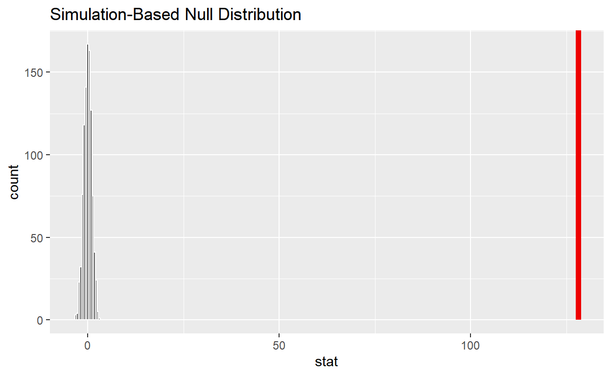
ggsave(filename = "preview.png", path = here::here("_posts", "2022-04-29-hypothesis-testing"))

Is the p-value < 0.05? yes
Does your analysis support the null hypothesis that the true means of the number of hours worked for those that were “fired”, “ok” and “promoted” were the same? no

Hypothesis Testing

Question: t-test

Question: Sample t-test 2

Question: ANOVA